Polygon Aperture
A 2D transverse aperture of a closed polygon defined by the \(x\) and \(y\) coordinates of the vertices. The vertices must be ordered in the counter-clockwise direction and must close, i.e. the first and last coordinates must be the same.
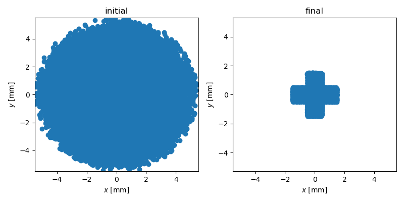
This example takes a 800 MeV proton beam generated as a waterbag distribution with \(\sigma_x\), \(\sigma_y\) both equal to 2 mm impinging directly the mask.
Several variations are given, with the mask either transmitting or blocking the particles, also with option rotation and transverse offset.
Run
This example of a transmitting mask can be run either as:
Python script:
python3 run_polygon_aperture.pyorImpactX executable using an input file:
impactx input_polygon_aperture.in
For MPI-parallel runs, prefix these lines with mpiexec -n 4 ... or srun -n 4 ..., depending on the system.
#!/usr/bin/env python3
#
# Copyright 2022-2023 ImpactX contributors
# Authors: Eric G. Stern, Axel Huebl, Chad Mitchell
# License: BSD-3-Clause-LBNL
#
# -*- coding: utf-8 -*-

from scipy.constants import c, eV, m_p

from impactx import ImpactX, distribution, elements

sim = ImpactX()

# set numerical parameters and IO control
sim.space_charge = False
# sim.diagnostics = False  # benchmarking
sim.slice_step_diagnostics = True

# domain decomposition & space charge mesh
sim.init_grids()

# load a 2 GeV electron beam with an initial
# unnormalized rms emittance of 2 nm
kin_energy_MeV = 800.0  # reference energy 800 MeV proton
bunch_charge_C = 1.0e-9  # used with space charge
npart = 50000  # number of macro particles

#   reference particle
ref = sim.particle_container().ref_particle()
ref.set_charge_qe(1.0).set_mass_MeV(1.0e-6 * m_p * c**2 / eV).set_kin_energy_MeV(
    kin_energy_MeV
)

#   particle bunch
distr = distribution.Waterbag(
    lambdaX=2.0e-3,
    lambdaY=2.0e-3,
    lambdaT=0.4,
    lambdaPx=4.0e-4,
    lambdaPy=4.0e-4,
    lambdaPt=2.0e-3,
    muxpx=0.0,
    muypy=0.0,
    mutpt=0.0,
)
sim.add_particles(bunch_charge_C, distr, npart)

# add beam diagnostics
monitor = elements.BeamMonitor("monitor", backend="h5")

vertices_x = [
    float(u)
    for u in "0.5e-3 0.5e-3 -0.5e-3 -0.5e-3 -1.5e-3 -1.5e-3 -0.5e-3 -0.5e-3 0.5e-3 0.5e-3 1.5e-3 1.5e-3 0.5e-3".split()
]
vertices_y = [
    float(u)
    for u in "0.5e-3 1.5e-3 1.5e-3 0.5e-3 0.5e-3 -0.5e-3 -0.5e-3 -1.5e-3 -1.5e-3 -0.5e-3 -0.5e-3 0.5e-3 0.5e-3".split()
]
mr2 = 2 * 0.5e-3**2

aperture = elements.PolygonAperture(vertices_x, vertices_y, action="transmit")

print(aperture.to_dict())
assert aperture.min_radius2 == 0.0
aperture.min_radius2 = mr2
assert abs(aperture.min_radius2 / mr2 - 1.0) < 1.0e-15

# design the accelerator lattice)
ns = 1  # number of slices per ds in the element
channel = [
    monitor,
    aperture,
    monitor,
]

sim.lattice.extend(channel)

# run simulation
sim.track_particles()

# clean shutdown
sim.finalize()
###############################################################################
# Particle Beam(s)
###############################################################################
beam.npart = 50000
beam.units = static
beam.kin_energy = 800.0
beam.charge = 1.0e-9
beam.particle = proton
beam.distribution = waterbag
beam.lambdaX = 2.0e-3
beam.lambdaY = beam.lambdaX
beam.lambdaT = 0.4
beam.lambdaPx = 4.0e-4
beam.lambdaPy = beam.lambdaPx
beam.lambdaPt = 2.0e-3
beam.muxpx = 0.0
beam.muypy = 0.0
beam.mutpt = 0.0


###############################################################################
# Beamline: lattice elements and segments
###############################################################################
lattice.elements = monitor pa monitor
lattice.nslice = 1

monitor.type = beam_monitor
monitor.backend = h5

pa.type = polygon_aperture
pa.vertices_x = 0.5e-3 0.5e-3 -0.5e-3 -0.5e-3 -1.5e-3 -1.5e-3 -0.5e-3 -0.5e-3 0.5e-3 0.5e-3 1.5e-3 1.5e-3 0.5e-3
pa.vertices_y = 0.5e-3 1.5e-3 1.5e-3 0.5e-3 0.5e-3 -0.5e-3 -0.5e-3 -1.5e-3 -1.5e-3 -0.5e-3 -0.5e-3 0.5e-3 0.5e-3
pa.min_radius2 = 5.0e-7
pa.action = "transmit" # this is the default transmit particles within the polygon
#pa.action = "absorb" # alternatively absorb particles within the polygon

###############################################################################
# Algorithms
###############################################################################
algo.space_charge = false


###############################################################################
# Diagnostics
###############################################################################
diag.slice_step_diagnostics = true
Other examples are
#!/usr/bin/env python3
#
# Copyright 2022-2023 ImpactX contributors
# Authors: Eric G. Stern, Axel Huebl, Chad Mitchell
# License: BSD-3-Clause-LBNL
#
# -*- coding: utf-8 -*-

from scipy.constants import c, eV, m_p

from impactx import ImpactX, distribution, elements

sim = ImpactX()

# set numerical parameters and IO control
sim.space_charge = False
# sim.diagnostics = False  # benchmarking
sim.slice_step_diagnostics = True

# domain decomposition & space charge mesh
sim.init_grids()

# load a 2 GeV electron beam with an initial
# unnormalized rms emittance of 2 nm
kin_energy_MeV = 800.0  # reference energy 800 MeV proton
bunch_charge_C = 1.0e-9  # used with space charge
npart = 50000  # number of macro particles

#   reference particle
ref = sim.particle_container().ref_particle()
ref.set_charge_qe(1.0).set_mass_MeV(1.0e-6 * m_p * c**2 / eV).set_kin_energy_MeV(
    kin_energy_MeV
)

#   particle bunch
distr = distribution.Waterbag(
    lambdaX=2.0e-3,
    lambdaY=2.0e-3,
    lambdaT=0.4,
    lambdaPx=4.0e-4,
    lambdaPy=4.0e-4,
    lambdaPt=2.0e-3,
    muxpx=0.0,
    muypy=0.0,
    mutpt=0.0,
)
sim.add_particles(bunch_charge_C, distr, npart)

# add beam diagnostics
monitor = elements.BeamMonitor("monitor", backend="h5")

vertices_x = [
    float(u)
    for u in "0.5e-3 0.5e-3 -0.5e-3 -0.5e-3 -1.5e-3 -1.5e-3 -0.5e-3 -0.5e-3 0.5e-3 0.5e-3 1.5e-3 1.5e-3 0.5e-3".split()
]
vertices_y = [
    float(u)
    for u in "0.5e-3 1.5e-3 1.5e-3 0.5e-3 0.5e-3 -0.5e-3 -0.5e-3 -1.5e-3 -1.5e-3 -0.5e-3 -0.5e-3 0.5e-3 0.5e-3".split()
]
mr2 = 2 * 0.5e-3**2

aperture = elements.PolygonAperture(vertices_x, vertices_y, action="absorb")

print(aperture.to_dict())
assert aperture.min_radius2 == 0.0
aperture.min_radius2 = mr2
assert abs(aperture.min_radius2 / mr2 - 1.0) < 1.0e-15

# design the accelerator lattice)
ns = 1  # number of slices per ds in the element
channel = [
    monitor,
    aperture,
    monitor,
]

sim.lattice.extend(channel)

# run simulation
sim.track_particles()

# clean shutdown
sim.finalize()
examples/polygon_aperture/run_polygon_aperture_absorb_rotate.py.#!/usr/bin/env python3
#
# Copyright 2022-2023 ImpactX contributors
# Authors: Eric G. Stern, Axel Huebl, Chad Mitchell
# License: BSD-3-Clause-LBNL
#
# -*- coding: utf-8 -*-
from scipy.constants import c, eV, m_p
from impactx import ImpactX, distribution, elements
sim = ImpactX()
# set numerical parameters and IO control
sim.space_charge = False
# sim.diagnostics = False # benchmarking
sim.slice_step_diagnostics = True
# domain decomposition & space charge mesh
sim.init_grids()
# load a 2 GeV electron beam with an initial
# unnormalized rms emittance of 2 nm
kin_energy_MeV = 800.0 # reference energy 800 MeV proton
bunch_charge_C = 1.0e-9 # used with space charge
npart = 50000 # number of macro particles
# reference particle
ref = sim.particle_container().ref_particle()
ref.set_charge_qe(1.0).set_mass_MeV(1.0e-6 * m_p * c**2 / eV).set_kin_energy_MeV(
kin_energy_MeV
)
# particle bunch
distr = distribution.Waterbag(
lambdaX=2.0e-3,
lambdaY=2.0e-3,
lambdaT=0.4,
lambdaPx=4.0e-4,
lambdaPy=4.0e-4,
lambdaPt=2.0e-3,
muxpx=0.0,
muypy=0.0,
mutpt=0.0,
)
sim.add_particles(bunch_charge_C, distr, npart)
# add beam diagnostics
monitor = elements.BeamMonitor("monitor", backend="h5")
vertices_x = [
float(u)
for u in "0.5e-3 0.5e-3 -0.5e-3 -0.5e-3 -1.5e-3 -1.5e-3 -0.5e-3 -0.5e-3 0.5e-3 0.5e-3 1.5e-3 1.5e-3 0.5e-3".split()
]
vertices_y = [
float(u)
for u in "0.5e-3 1.5e-3 1.5e-3 0.5e-3 0.5e-3 -0.5e-3 -0.5e-3 -1.5e-3 -1.5e-3 -0.5e-3 -0.5e-3 0.5e-3 0.5e-3".split()
]
mr2 = 2 * 0.5e-3**2
aperture = elements.PolygonAperture(
vertices_x, vertices_y, action="absorb", rotation=30.0
)
print(aperture.to_dict())
assert aperture.min_radius2 == 0.0
aperture.min_radius2 = mr2
assert abs(aperture.min_radius2 / mr2 - 1.0) < 1.0e-15
# design the accelerator lattice)
ns = 1 # number of slices per ds in the element
channel = [
monitor,
aperture,
monitor,
]
sim.lattice.extend(channel)
# run simulation
sim.track_particles()
# clean shutdown
sim.finalize()
#!/usr/bin/env python3
#
# Copyright 2022-2023 ImpactX contributors
# Authors: Eric G. Stern, Axel Huebl, Chad Mitchell
# License: BSD-3-Clause-LBNL
#
# -*- coding: utf-8 -*-

from scipy.constants import c, eV, m_p

from impactx import ImpactX, distribution, elements

sim = ImpactX()

# set numerical parameters and IO control
sim.space_charge = False
# sim.diagnostics = False  # benchmarking
sim.slice_step_diagnostics = True

# domain decomposition & space charge mesh
sim.init_grids()

# load a 2 GeV electron beam with an initial
# unnormalized rms emittance of 2 nm
kin_energy_MeV = 800.0  # reference energy 800 MeV proton
bunch_charge_C = 1.0e-9  # used with space charge
npart = 50000  # number of macro particles

#   reference particle
ref = sim.particle_container().ref_particle()
ref.set_charge_qe(1.0).set_mass_MeV(1.0e-6 * m_p * c**2 / eV).set_kin_energy_MeV(
    kin_energy_MeV
)

#   particle bunch
distr = distribution.Waterbag(
    lambdaX=2.0e-3,
    lambdaY=2.0e-3,
    lambdaT=0.4,
    lambdaPx=4.0e-4,
    lambdaPy=4.0e-4,
    lambdaPt=2.0e-3,
    muxpx=0.0,
    muypy=0.0,
    mutpt=0.0,
)
sim.add_particles(bunch_charge_C, distr, npart)

# add beam diagnostics
monitor = elements.BeamMonitor("monitor", backend="h5")

vertices_x = [
    float(u)
    for u in "0.5e-3 0.5e-3 -0.5e-3 -0.5e-3 -1.5e-3 -1.5e-3 -0.5e-3 -0.5e-3 0.5e-3 0.5e-3 1.5e-3 1.5e-3 0.5e-3".split()
]
vertices_y = [
    float(u)
    for u in "0.5e-3 1.5e-3 1.5e-3 0.5e-3 0.5e-3 -0.5e-3 -0.5e-3 -1.5e-3 -1.5e-3 -0.5e-3 -0.5e-3 0.5e-3 0.5e-3".split()
]
mr2 = 2 * 0.5e-3**2

aperture = elements.PolygonAperture(
    vertices_x, vertices_y, action="absorb", dx=0.0006, dy=-0.0012
)

print(aperture.to_dict())
assert aperture.min_radius2 == 0.0
aperture.min_radius2 = mr2
assert abs(aperture.min_radius2 / mr2 - 1.0) < 1.0e-15

# design the accelerator lattice)
ns = 1  # number of slices per ds in the element
channel = [
    monitor,
    aperture,
    monitor,
]

sim.lattice.extend(channel)

# run simulation
sim.track_particles()

# clean shutdown
sim.finalize()
examples/polygon_aperture/run_polygon_aperture_absorb_rotate_offset.py.#!/usr/bin/env python3
#
# Copyright 2022-2023 ImpactX contributors
# Authors: Eric G. Stern, Axel Huebl, Chad Mitchell
# License: BSD-3-Clause-LBNL
#
# -*- coding: utf-8 -*-
from scipy.constants import c, eV, m_p
from impactx import ImpactX, distribution, elements
sim = ImpactX()
# set numerical parameters and IO control
sim.space_charge = False
# sim.diagnostics = False # benchmarking
sim.slice_step_diagnostics = True
# domain decomposition & space charge mesh
sim.init_grids()
# load a 2 GeV electron beam with an initial
# unnormalized rms emittance of 2 nm
kin_energy_MeV = 800.0 # reference energy 800 MeV proton
bunch_charge_C = 1.0e-9 # used with space charge
npart = 50000 # number of macro particles
# reference particle
ref = sim.particle_container().ref_particle()
ref.set_charge_qe(1.0).set_mass_MeV(1.0e-6 * m_p * c**2 / eV).set_kin_energy_MeV(
kin_energy_MeV
)
# particle bunch
distr = distribution.Waterbag(
lambdaX=2.0e-3,
lambdaY=2.0e-3,
lambdaT=0.4,
lambdaPx=4.0e-4,
lambdaPy=4.0e-4,
lambdaPt=2.0e-3,
muxpx=0.0,
muypy=0.0,
mutpt=0.0,
)
sim.add_particles(bunch_charge_C, distr, npart)
# add beam diagnostics
monitor = elements.BeamMonitor("monitor", backend="h5")
vertices_x = [
float(u)
for u in "0.5e-3 0.5e-3 -0.5e-3 -0.5e-3 -1.5e-3 -1.5e-3 -0.5e-3 -0.5e-3 0.5e-3 0.5e-3 1.5e-3 1.5e-3 0.5e-3".split()
]
vertices_y = [
float(u)
for u in "0.5e-3 1.5e-3 1.5e-3 0.5e-3 0.5e-3 -0.5e-3 -0.5e-3 -1.5e-3 -1.5e-3 -0.5e-3 -0.5e-3 0.5e-3 0.5e-3".split()
]
mr2 = 2 * 0.5e-3**2
aperture = elements.PolygonAperture(
vertices_x, vertices_y, action="absorb", dx=0.0006, dy=-0.0012, rotation=30.0
)
print(aperture.to_dict())
assert aperture.min_radius2 == 0.0
aperture.min_radius2 = mr2
assert abs(aperture.min_radius2 / mr2 - 1.0) < 1.0e-15
# design the accelerator lattice)
ns = 1 # number of slices per ds in the element
channel = [
monitor,
aperture,
monitor,
]
sim.lattice.extend(channel)
# run simulation
sim.track_particles()
# clean shutdown
sim.finalize()
Analyze
We run the following script to analyze correctness:
Script analysis_polygon_aperture.py
#!/usr/bin/env python3
#
# Copyright 2022-2023 ImpactX contributors
# Authors: Eric G. Stern, Axel Huebl, Chad Mitchell
# License: BSD-3-Clause-LBNL
#


import numpy as np
import openpmd_api as io

# initial/final beam
series = io.Series("diags/openPMD/monitor.h5", io.Access.read_only)
last_step = list(series.iterations)[-1]
initial = series.iterations[1].particles["beam"].to_df()
beam_final = series.iterations[last_step].particles["beam"]
final = beam_final.to_df()

# compare number of particles
num_particles = len(initial.momentum_x)
assert num_particles == len(initial)
assert num_particles != len(final)

print("Initial Beam: ", len(initial), " particles")
print("Final Beam: ", len(final), " particles")

# Make sure no particles are outside of the aperture in the final particle set
abs_x_final = abs(final["position_x"]).to_numpy()
abs_y_final = abs(final["position_y"]).to_numpy()

N = abs_x_final.shape[0]
insides = np.zeros(N, dtype=np.bool)
for i in range(N):
    insides[i] = ((abs_y_final[i] < 0.5e-3) and (abs_x_final[i] < 1.5e-3)) or (
        (abs_x_final[i] < 0.5e-3) and (abs_y_final[i] < 1.5e-3)
    )


outsides = ~insides
ninside = insides.sum()
noutside = outsides.sum()

assert ninside == len(final)
assert noutside == 0
The number of surviving particles is printed and checked.
Visualize
You can run the following script to visualize aperture effect:
Script plot_polygon_aperture.py
#!/usr/bin/env python3
#
# Copyright 2022-2025 ImpactX contributors
# Authors: Eric G. Stern, Axel Huebl, Chad Mitchell
# License: BSD-3-Clause-LBNL
#

import argparse

import matplotlib.pyplot as plt
import openpmd_api as io

# options to run this script
parser = argparse.ArgumentParser(description="Plot action of the polygon aperture.")
parser.add_argument(
    "--save-png", action="store_true", help="non-interactive run: save to PNGs"
)
args = parser.parse_args()


# initial/final beam
series = io.Series("diags/openPMD/monitor.h5", io.Access.read_only)
last_step = list(series.iterations)[-1]
initial = series.iterations[1].particles["beam"].to_df()
final = series.iterations[last_step].particles["beam"].to_df()


f, axs = plt.subplots(1, 2, figsize=(8, 4), constrained_layout=True)

axs[0].scatter(initial["position_x"] * 1.0e3, initial["position_y"] * 1.0e3)
axs[0].set_title("initial")
axs[0].set_xlabel(r"$x$ [mm]")
axs[0].set_ylabel(r"$y$ [mm]")
axs[0].set_xlim([-5.5, 5.5])
axs[0].set_ylim([-5.5, 5.5])

axs[1].scatter(final["position_x"] * 1.0e3, final["position_y"] * 1.0e3)
axs[1].set_title("final")
axs[1].set_xlabel(r"$x$ [mm]")
axs[1].set_ylabel(r"$y$ [mm]")
axs[1].set_xlim([-5.5, 5.5])
axs[1].set_ylim([-5.3, 5.3])


plt.tight_layout()
if args.save_png:
    plt.savefig("polygon_aperture.png")
else:
    plt.show()